Create a PivotTable Calculated Item in Excel

Excel’s PivotTable feature allows you to organize information in such a way that you can answer many questions about your data that would otherwise require lots of formulas, functions and “IF” statements. To get even more answers out of your data, PivotTables offer Calculated Fields and Calculated Items.

• Calculated Fields allow you to use existing PivotTable fields in a formula or calculation.
• Calculated Items allow you to create a new item or category in an existing PivotTable field, combining other items and categories into formulas or custom calculations.

This article will describe how to create a PivotTable Calculated Item.

Start by creating a PivotTable from the source data you want analyzed. Our example will analyze sales data by item and category. These steps apply to Excel 2010-2013, though the specific steps may vary based on your version. Images were taken using Excel 2013 on the Windows 7 OS.

To follow using our example, download Create a PivotTable Calculated item.xlsx

Create a Calculated Item

1. Select any item in your PivotTable, then click the Fields, items, & Sets button in the Calculations group on the Analyze Choose Calculated Item from the dropdown menu.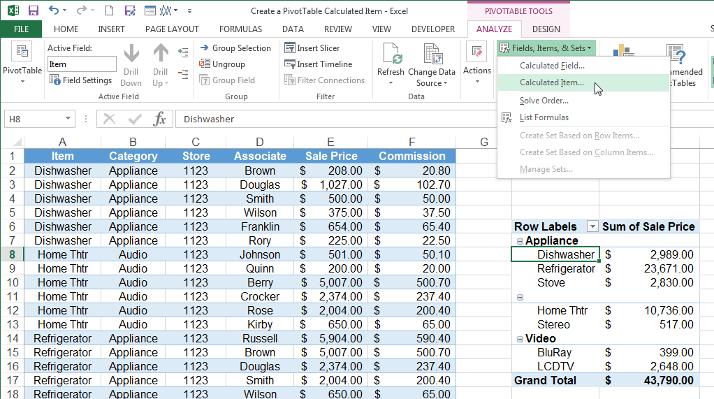

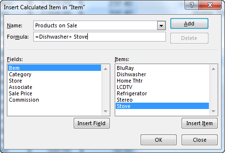
2. We know that certain products were on sale during the month that the data represents. We would like to see a summary of all sale items in our PivotTable. To that end, we will create a new Calculated Item called “Products on Sale” that combines the sale products into one field.

Note: In Excel 2010, Calculated Item menu option is found under PivotTable Tools > Options Tab > Fields, Items, & Sets

• Type a name for the new field in the Name
• Select the field that contains the items you wish to manipulate in the Fields selection box and add it to the Formula by clicking Insert Field or Insert Items within the field into the Formula box.
• Click OK when the formula is complete.

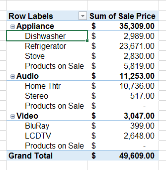
3. The “Products on Sale” item will be added to each category in the PivotTable.

Hint: Note that in this setup the PivotTable automatically subtotaled the Sales Categories, including the new “Products on Sale” item. This means that the items that appear in both Dishwasher and Stove are counted twice in this subtotal and Grand Total.

To avoid confusion, you can:

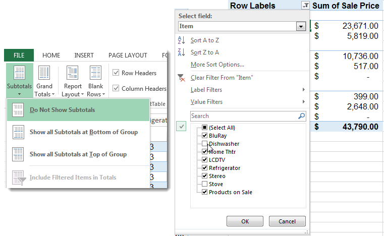
• Turn off subtotals in the Subtotals dropdown menu in the Layout group on the Design Turn off Grand Totals in the same way from the Grand Totals dropdown menu.
• Take out the items that are duplicated by de-selecting them in the Row Labels filter dropdown.

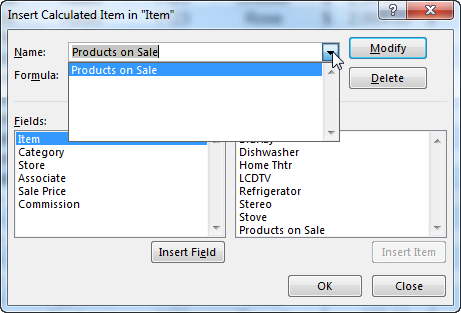
4. To delete a calculated item, click on the Fields, items, & Sets button in the Calculations group on the Analyze tab (Options tab in Excel 2010). Choose Calculated Item from the dropdown menu just like you did to create it. Then, select the calculated item from the dropdown menu in the Name textbox and click the Delete button.

Calculated items can be trickier to work with as they cannot be moved into the Report Filters area of the PivotTable and you have to be careful if the item creates duplicate entries in the totals as described above. However, it can be a useful feature when you want to analyze your information by broader categories than a calculated field can work with easily.

Visit this blog post to learn How to Create a PivotTable Calculated Field in Excel.