Create an Excel Pivot Chart from Your PivotTable

Problem:  You have data with thousands of donors and their annual gifts listed. The PivotTable you are using still doesn’t help you see which donors gave the most or how many donors gave you donations at various giving tiers.

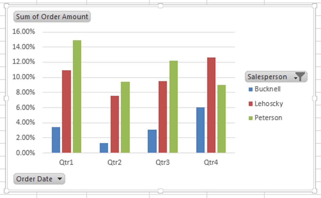
Solution:  Create a PivotChart. You may need a visual representation of PivotTable information for a PowerPoint slide, a meeting agenda, a report, or faster analysis. A PivotChart gives you the snapshot of that data that you need like a traditional chart, but also adds interactive filtering controls directly from the PivotChart so you can quickly analyze different slices of your data.

What Microsoft Calls It: Insert a PivotChart

Create a PivotChart

There are two ways you can create a PivotChart in Excel 2013. The first takes advantage of Excel’s Recommended Charts tool. When you use this feature, you do not need to create a PivotTable first in order to create and use a PivotChart.

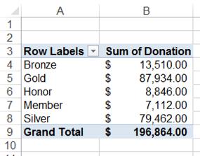
You can also create a PivotChart from an already existing PivotTable, making use of the filters and fields you have already organized.

Step-by-Step

Option 1 – Create a PivotChart from Recommended Charts

1. Select the data you want to chart.

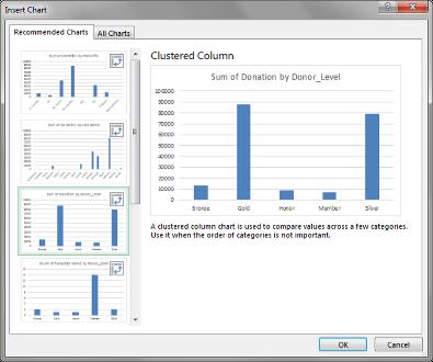
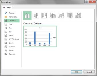
2. Click the Recommended Charts button in the Charts group on the Insert tab to open the Insert Chart dialog box.

3.  The Insert Chart dialog box will open to the Recommended Charts tab where a list of sample charts will be offered in the menu on the left side. A PivotChart icon in the upper right corner of the option indicates that the chart is a PivotChart.  

4. Click on any recommended chart to view a preview of the table in the Preview Pane.

5. When you have chosen a chart that meets your needs (or almost meets your needs), click OK.

The PivotChart (and a companion PivotTable) will be created in a new worksheet to the left of the one where your data was selected.

If none of the recommended charts are satisfactory, close the Insert Chart dialog box and follow the steps in Option 2 to create a PivotChart from scratch.

Step-by-Step

Option 2 – Create a PivotChart from an existing PivotTable

1. Click anywhere in the PivotTable to activate the PivotTable Tools contextual tabs.

2. Click the PivotChart button in the Tools group on the Analyze tab to open the Insert Chart dialog box. 3. Choose the type of chart you want from the left side menu. Choose chart options from the top menu. Preview your PivotChart in the preview pane.

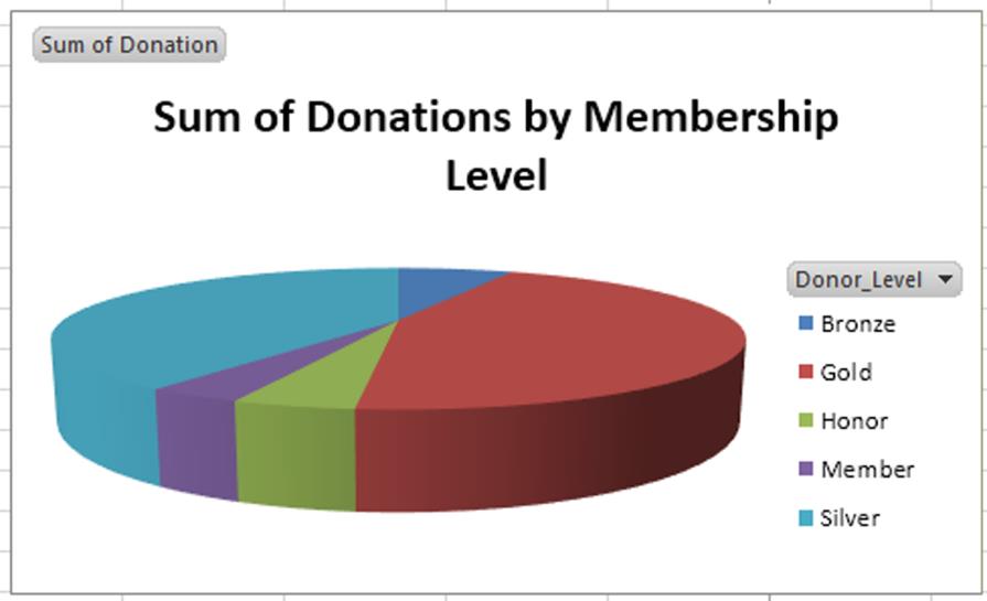
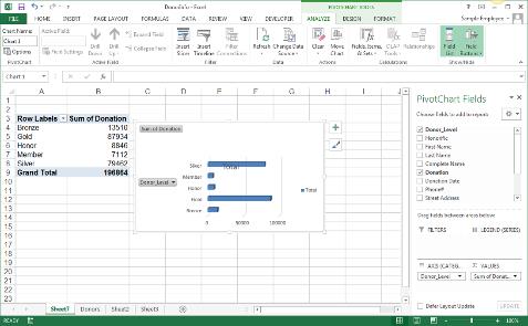
4. Click OK to enter the PivotChart into the worksheet where the PivotTable was selected.

5. When your PivotChart has been created, you can make edits to the chart elements and colors by making changes in the PivotChart Fields list or clicking the Chart Elements and Chart Styles buttons.

6. Review your PivotChart. You can change chart filters directly from the Interactive Controls [L] on the PivotChart to see different slices of your data.