Create Outstanding Pie Charts in Excel
Once you have gone to the effort of collecting, organizing and processing your data, you probably want to show it off! Tables do a nice job of presenting raw information, but a chart can bring your data to life. Charts create visual impact that conveys not only the data itself, but its relationships and meaning.
The Pie Chart is an “industry standard” for conveying the relationship of parts to the whole. You will use pie charts when you want to show how specific aspects – or slices – of your data contribute to the big picture. Pie charts are not good for showing changes over time. You also won’t use a pie chart when you need to compare data that is not, in the end, summarized into a grand total.
The following steps illustrate how to add a pie chart to your Excel spreadsheet. These steps apply to Excel 2007-2013. Images were taken using Excel 2013 on the Windows 7 OS so the specific steps may vary based on your version.
To follow using our example, download Excel Pie Chart Tutorial.xlsx: Insert the chart
Insert the Chart
In our example, we want to show the relationship between the different levels of donors that give to our charity as compared to total giving. A pie chart is perfect for this illustration. We will start with a summary of the giving totals by level.
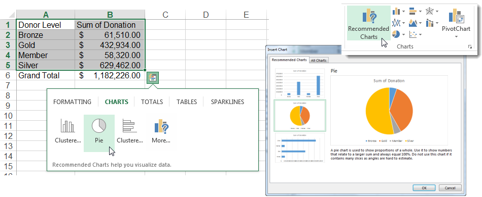
- Select the range or table of data you want to illustrate in your chart. (Note that if your table has a “Grand Total” row, do NOT include this row or it will be considered a “slice” of your pie.)
- On the Insert tab, click the Pie chart icon in the Charts There are several default charts to choose from. Hover over an option to see a preview of the chart, then select the one that is closest to what you want.

Hint! If you are using Excel 2013 or higher, you can click on the Recommended Charts option that appears in the Quick Analysis tool icon beside your data. Or, you can click the Recommended Charts button in the Charts group to open the Recommended Charts tab on the Insert Chart dialog box.
Edit Your Pie Chart
To follow using our example, download Excel Pie Chart Tutorial.xlsx: Edit Your Pie Chart Examples
Once your basic chart is in place, you will have details you need to add, change or style. Click on the chart that you wish to modify to activate the Chart Tools contextual tabs and edit buttons. (You can make many changes directly from the chart’s edit buttons in Excel 2013).
On the Design Tab
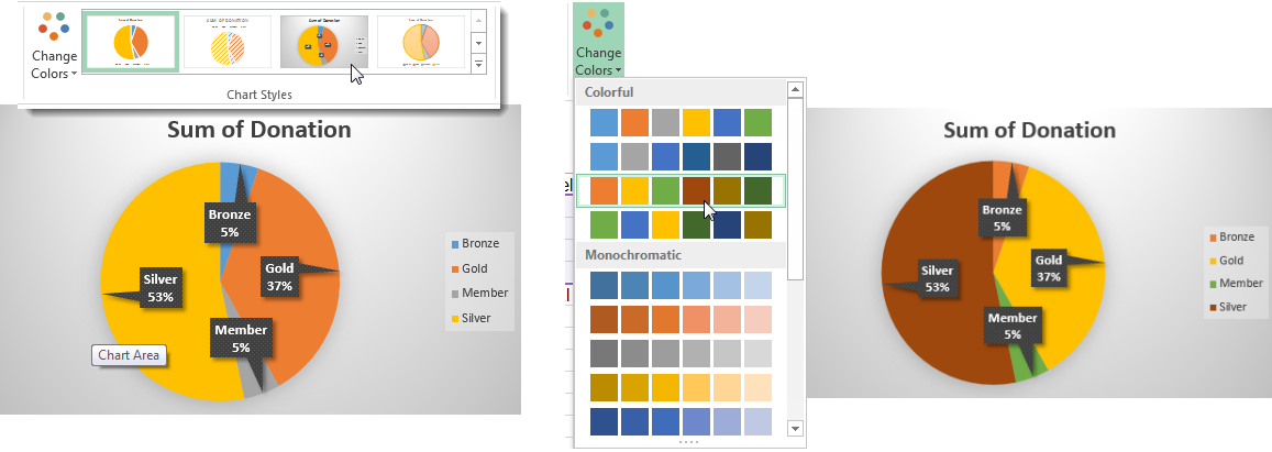
- Add data labels, adjust the Chart Title and Legend. Click “More…Options” to open the Format Pane to access even more settings.
- Change the Chart Style or Chart Colors.
On the Format Tab
- Edit and style text in the Title, Legend, etc.
- Drag individual elements on the chart to new locations.
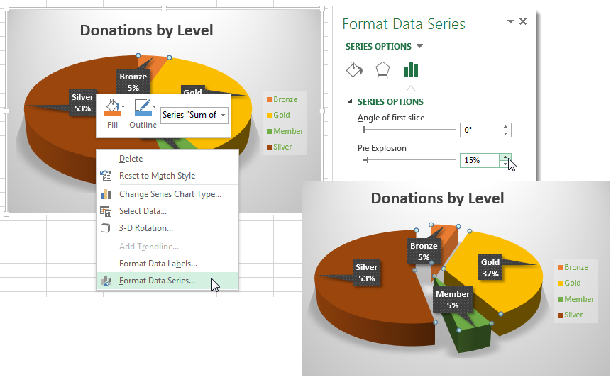
- “Explode” the slices:
- To separate an individual slice, simply select it and drag it away from the chart.
- To pull all slices away from the center, right-click on the chart and select Format Data Series. In the Format Data Series pane, click the Pie Explosion slider to adjust the distance between pieces.
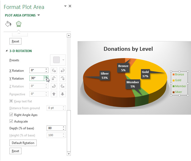
- If your pie chart is a 3D chart, you can format thickness, rotation, and add shadows, and more to the Chart and Plot Area.
When you are finished, you will not only have an informative illustration of how much each group of donors contributes to the organization, you also have a beautifully designed graphic that will fit into brochures, posters and online content in the colors and style of your organization’s branding.
To see the finished product, download Excel Pie Chart Tutorial.xlsx: Finished Product


