Excel PivotTable Formulas

It’s easy to create formulas with PivotTable data. The key is to remember that you are working with aggregate values, not individual ones. We’ll take a look at how to create a simple formula using something called a Calculated Field. And then, we’ll take a look at two common causes of confusion and errors with PivotTable calculations.

Download Excel Pivot Table Formulas.xlsx to follow along with the instructions.

Creating a Calculated Field

In our example, we’ve created a PivotTable from our source data which contains the following columns.

• Product
• Customer
• Warehouse 1 – dollar value of product shipped from Warehouse 1 this year
• Warehouse 2 – dollar value of product shipped from Warehouse 2 this year
• Warehouse 3 – dollar value of product shipped from Warehouse 3 this year
• Warehouse 4 – dollar value of product shipped from Warehouse 4 this year
• Previous Year Total – dollar value of products shipped from all warehouses last year
• % Previous Year Total – A formula yielding the sum of this year’s total shipments over the previous year’s total.

We can create a calculated field equaling the sum of all warehouse shipments for each product with the following steps.

1. Add a row field to the PivotTable report area to make the Fields, Items & Sets button active in Calculations group on the Analyze tab.
2. Click the Fields, Items & Sets button and select Calculated Field.

Note: Do not select Calculated Item! This does a different type of aggregation.

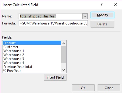
3. Name the field “Total Shipped This Year.”
4. In the Formula field, type =SUM(.
5. Below, in the Fields section, select each Warehouse # field and then click the Insert Field button, inputting a comma between each field name.
6. Click OK.
7. This new calculated field is now added to your PivotTable.

If you had other PivotTables in your workbook based on this same Source Data, all of them would have this new calculated field added to the field list.

Formulas Next to PivotTables

“Why couldn’t I just have put that SUM function right next to the PivotTable?” you may be asking. Well, unlike regular formulas which refer to a cell reference (column and row), the default behavior of PivotTable values is as a “data point” or aggregate total. You might see something like this when you try to add a formula next to your PivotTable:

=GETPIVOTDATA(“Sum of Warehouse 1″,$A$3,”Product”,”Alice Mutton”)
This is referring to the aggregate data point made up of all Warehouse 1 values for the Product Alice Mutton, and NOT what is in cell B4. If we sort the PivotTable in reverse order by product, your GETPIVOTDATA statement doesn’t change and still refers to that same data point. You could type in the cell reference, so =B4, instead of just clicking on the cell, but as your PivotTable changes in length some of those formulas may refer to empty cells.

You can turn the GETPIVOTDATA feature off on the Analyze tab, by clicking the drop down arrow next to the Options button and clicking the check mark off of Generate GetPivotData.

Aggregate vs. Individual Values

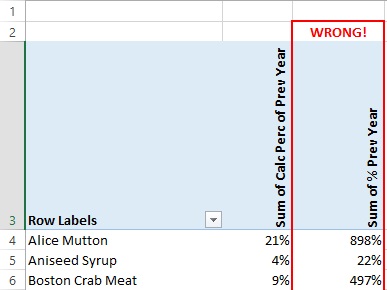
What if instead of using the % Prev Year column, we created a calculated field for this number. Let’s see if things match up.

Well, obviously they don’t! Our calculated field is correct. The other field which was already in our Source Data simply added up all of the percentage numbers. It is important to know whether calculations should be done as calculated fields in the PivotTable or simply as an additional column in the source data. Try it out and practice with your pivot data.