Finding Information with the Index Formula in Excel

About Excel’s INDEX Function

Sometimes useful functions like VLOOKUP just don’t apply when the information you need is more about where in your table the information is than what the information is. The INDEX function returns the value of an element that is specified by position (row and column) in an array or table. You might use INDEX to:

• Get the “Nth” item from a list
• Get all values in a row or column

You can specify a certain range of cells to search using the Range Format of the function:

syntax: INDEX( range, row_num, [col_num], [area_num] )
Or, you can specify a certain range of cells to search using the Array Format of the function:

syntax: INDEX( array, row_num, [col_num] )
Often you will use INDEX when you want to create a form that allows you to get data based on a variable that you input manually. Combined with other functions into Excel formulas, INDEX can be quite robust. In this article, we will look at two simple examples of the INDEX function to show the basic idea. Steps below apply to Excel 2007 and later. Images were taken using Excel 2013 on Windows 7 – specific steps may vary based on your version.

To follow using our example, download Excel Formula Index.xlsx sheet: Get item from list

Use INDEX to get the “Nth” item from a list

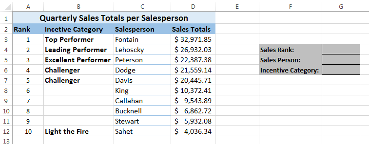
In this example, we want to reward the top performers on our sales team and motivate the rest to improve. As such, we need to know who is ranked 1^st, 2^nd, 3^rd and last, etc. for the quarter so we can send that salesperson customized rewards and messaging. We want to type in the rank (1-10) and have our form return the name and incentive category for that ranking.

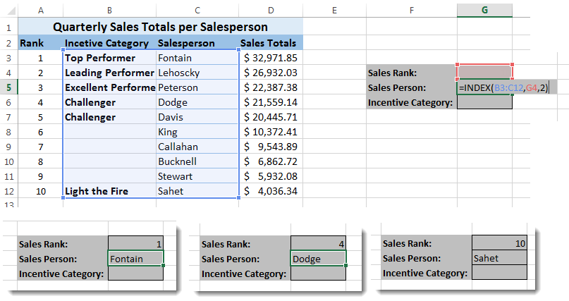
The formula we will put in cell G5 to accomplish this is: =INDEX(B3:C12,G4,2)

• B3:C12 describes our range. Notice that we exclude column and row headings so we can easily request 1^st place and so on without counting offset rows in our sheet.
• G4 tells the function to use the value in that cell to identify the row number to return.
• 2 tells the function to use the 2^nd column in the range to return.

Now you can type in a rank from 1-10 in G4 and return the correct salesperson.

The formula to return the Incentive Category is very similar. You will simply change the column number:  =INDEX(B3:C12,G4,1)

Use INDEX to get all values in a row or column

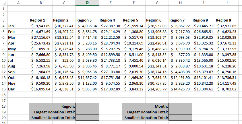
We want to discover the minimum and maximum donation amounts for each region and month in our organization. By combining INDEX into an Excel formula, we can create simple to complex analysis of our data.

To follow using our example, download Excel Formula Index.xlsx sheet: Get all items in row or column.

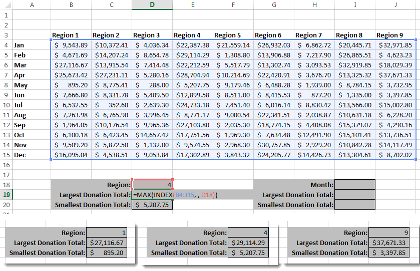
To calculate the largest donation for a specified region, the formula we would put in cell D19 is:

=MAX(INDEX(B4:J15, , D18))

• B4:J15 describes our range. Notice that we exclude column and row headings so we can easily request region and month with a simple number instead of counting offset rows in our sheet.
• The empty column argument “, ,” tells the function to get all values in the column (Zero can also be used)
• D18 tells the function to use the value in that cell to identify the row number to return.

To calculate the smallest regional donation, the formula we would put in cell D20 is:

=MIN(INDEX(B4:J15, , D18))

To calculate MIN and MAX for each month, we would use a similar formula and tell the INDEX function to get an entire row of information instead of an entire column. The formulas in I19 and I20 would look like this:

=MAX(INDEX(B4:J15,I18, 0))

=MIN(INDEX(B4:J15,I18, 0))

Wait! Can’t you just get this information with a simple MIN or MAX formula at the end of each row or column?

The answer is, of course, yes. For this simple example, INDEX is a bit “overkill”. However, when you begin creating complex formulas, the ability of the INDEX function to pluck data from a cell or range can save you time and your processor computing power.