How to Calculate Median in an Excel PivotTable – Almost!

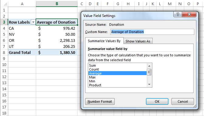
A frequent question that comes up when working with Excel PivotTables is how to calculate median using the table’s filters and analysis. The short answer is “Excel doesn’t do that”. Meaning, there isn’t a simple way to change the Value Field Settings to calculate “Median”. The closest you can get is “Average”.

However, averages aren’t always the best way to understand your data. Our example shows donations collected by a regional charity. Most of the donations are small amounts, a handful are more significant, and one or two are very large. The average donation for the year is $1380.50, but that does not accurately show us how most of our donors give. The median calculation shows us that most of our donations are around $50 with half giving more, and half giving less. This number more realistically reveals our donor giving patterns.

Images in this article were taken using Excel 2013 on the Windows 7 OS. To follow using our example below, download Calculate Median in PivotTables.xlsx

If we want to understand our donor giving patterns by state, we would naturally turn to a PivotTable and get something like we see in the first image. But what if we want the median donation for each state?

Here is the first of two “workaround” solutions to get a median calculation out of your PivotTable information. As with all workarounds, it may not be elegant, but it can get you started. The steps demonstrated will apply to Excel 2010 and later.

Use the Array Feature

Technically, the end result isn’t a PivotTable, but you can use the PivotTable feature to set up your array more easily:

1. First, create a PivotTable with the data organized in the way you want except with an Average calculation instead of Median in the Values area.

2. Then, select the PivotTable cells (headings included) and hit Ctrl+C to copy the table to your clipboard.

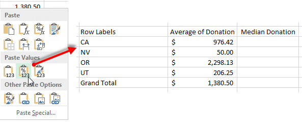
3. Right-click on an open cell and select Paste Special > Paste Values to paste a copy of the table’s headers and values in your worksheet.

4. Add a column to the new table for the Median calculation.

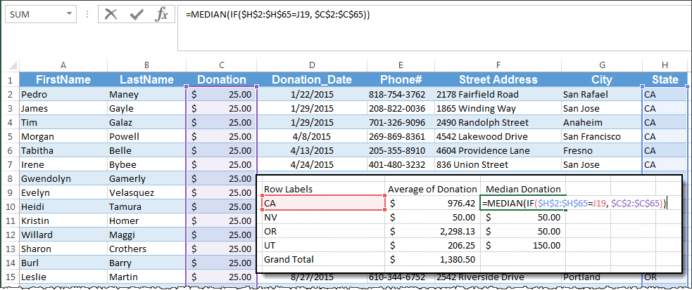
5. For each Row Label, combine the IF function with the MEDIAN function to pull only the data that corresponds to the fields in the PivotTable. Type the formula in the Median column. In our example, the formula will look like:

1. • =MEDIAN( tells Excel to calculate the median of the numbers that the IF statement returns
   • IF(($H$2:$H$65=J19, tells Excel to only return donor amount values if the value in the H column – State – matches the value in the J column (our PivotTable State Row Label). Use the $ symbol to specify absolute cell values.
   • $C$2:$C$65)) tells Excel to return the values in the C column that meet the above criteria for the MEDIAN function. Use the $ symbol to specify absolute cell values.
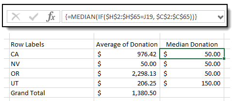
   • Hit Ctrl+Shift+Enter Important! Don’t just hit enter to complete the formula. You must hold Ctrl+Shift+Enter down together to complete the formula and tell Excel that it is an array formula. Excel will add curly braces around the formula if this is done correctly:

6. Now you can drag the formula to the other cells in the “fake” PivotTable and quickly see the Median Donation for all States covered by the charity.

So, “this isn’t really a PivotTable”, but this method does allow you to quickly harness the visual power of PivotTables to organize your information. You still have to do the manual work of making the Median calculation, but the PivotTable step gives you a shortcut to organizing your information and creating the formula. And until Microsoft adds the MEDIAN function directly to PivotTables, this is the most common solution out there.