How to Add Calculated Fields to a PivotTable in Excel

PivotTables are great tools for grouping, summarizing and totaling information from raw data. Once you have created a table, then you are ready to get even more out of your information by using the summarized data in additional formulas or calculations. The way Excel does this is through Calculated Fields.

These features apply to Excel 2007-2013, though the specific steps may vary based on your version. Images were taken using Excel 2013 on the Windows 7 OS. To follow using our example, download Create a PivotTable Calculated Field.

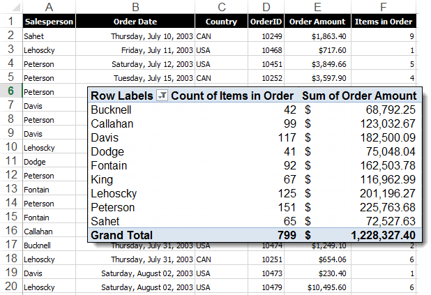
1. Click on any field in the PivotTable you want to enhance to open the PivotTable Tools contextual tab and the PivotTable Fields In this example, we have information about how much each of our salespeople have sold, and how many items were sold. We would like to know the average price of items sold to discover which sales members are doing best at selling higher priced items.
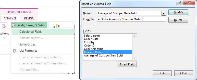
2. Click the Fields, Items, & Sets button in the Calculations group of the Analyze tab in the highlighted PivotTable Tools contextual tab then select Calculated Field.
3. In the Insert Calculated Field dialog box, type a descriptive name for your new field in the Name: textbox then type your formula using the Fields selection box to insert the fields that will be used in the calculation. In this example, we want to divide the “Order Amount” field by the “Items in Order” field to get the cost of the average item sold.
4. Click the OK button.

The results in the last column show that Dodge and Fontain sell more high-price items than Sahet and Callahan.

Calculated fields give you a way to add more value to your analysis without jumping through hoops in your source spreadsheets.

Bonus Hint:

Before you go through a lot of formula gymnastics to create a calculated field that will return results that show percentages of total or difference in total over time, check the Value Field Settings dialog box first.

To access the Value Field Settings dialog box, click anywhere in the column you want to change, then click on the Field Settings button in the Active Field group on the Analyze contextual tab OR double-click on the column heading.

This handy tool allows you to change the way your data is displayed in your PivotTable without writing formulas. For example:

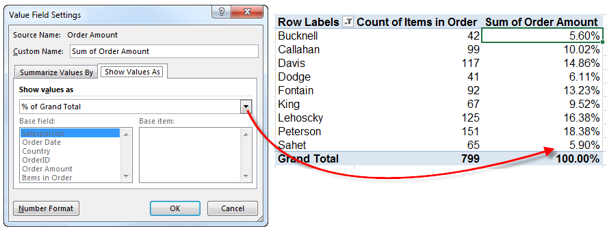
• Select Show Values As “% of Grand Total” to see how each salesperson is contributing to the bottom line:
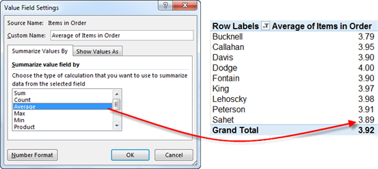
• Summarize item values by Average so you can see the average number of items in each salesperson’s order without creating a separate calculation (be sure to put your cursor on the field you want to average):

Visit this blog post to learn how to Create a PivotTable Calculated Item in Excel.