How to Create PivotTables Using the Quick Analysis Tool in Excel

Storing information is only part of the useful things Excel spreadsheets can do. Once you have collected a set of data, Excel can help you organize it and analyze it. One of the most powerful tools for analysis is the PivotTable. PivotTables do more than generate graphs out of one or two data points. When used to their full potential, PivotTables can:

• Reveal trends
• Expose performance (or lack thereof)
• Quickly summarize and compare variations in data groupings

But with all that flexibility, PivotTables can be somewhat intimidating to implement. The developers at Microsoft Office offered some help for that in Excel 2013. The steps below will demonstrate how to create PivotTables using Excel’s Quick Analysis Tool and will apply only to Excel 2013 or later. Images in this article were taken using Excel 2013 on the Windows 7 OS. To follow using our example below, download Create a PivotTable.xlsx

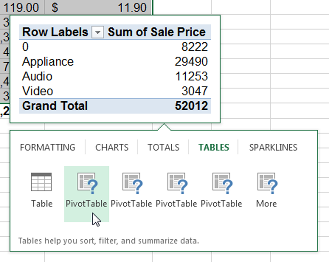
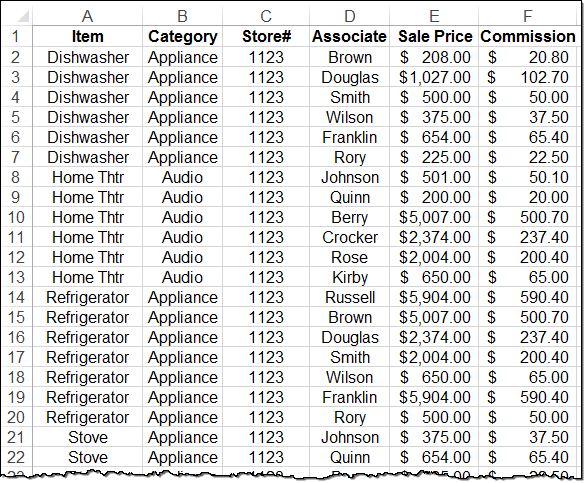
1. Open the sheet with the data you want to analyze. Highlight the data you want to include in the PivotTable. When you do so, the Quick Analysis Tool icon will appear in the bottom right corner of the selection.
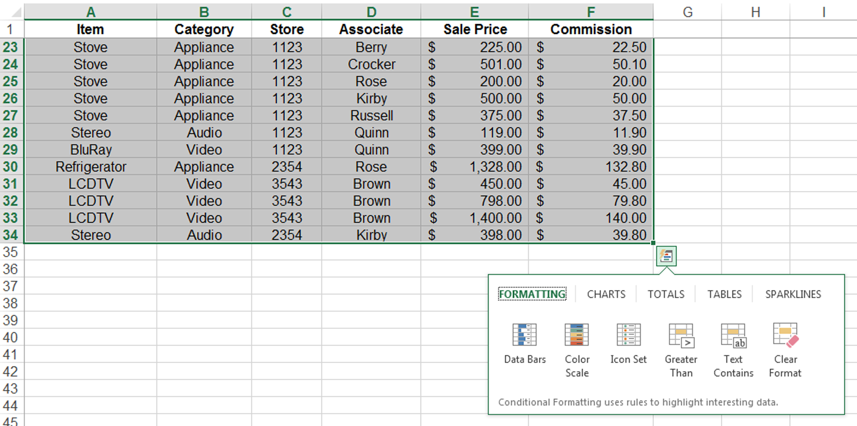
2. Click the icon to open the menu, then click Tables from the top row of menu options. Hover over any PivotTable option to see if any are similar to the type of table you are looking for. If it is, click it to create the table.

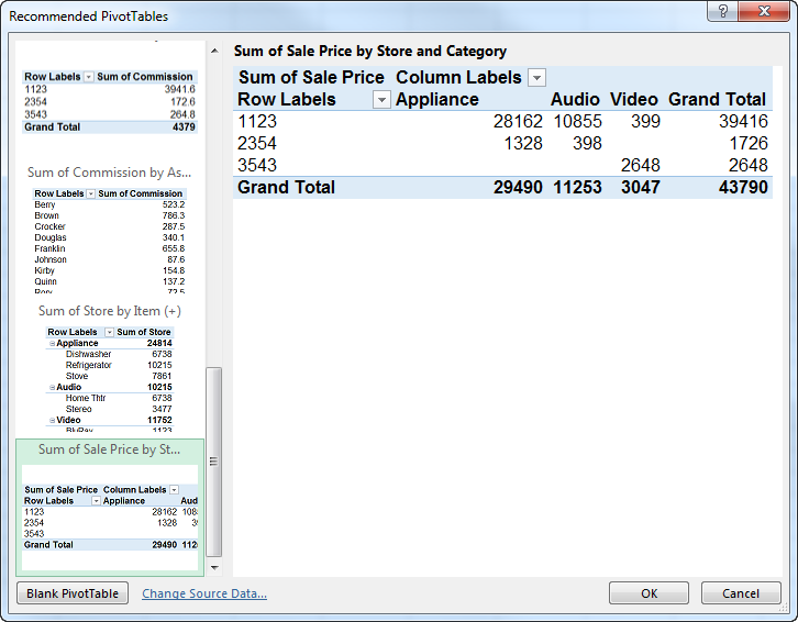
If you would like more options, click More to open the Recommended PivotTables dialog box. From this window you can select and preview several different PivotTable options. Click OK when you find the one you want.

The Recommended PivotTables show you several ways to sort and analyze your data and can be a useful tool in itself! Using our source data:

You can learn several different things about how your stores are performing such as:

• Which stores perform best in different product lines (Appliance, Audio, Video) and which perform best overall:

• Which sales people are earning the most commission:

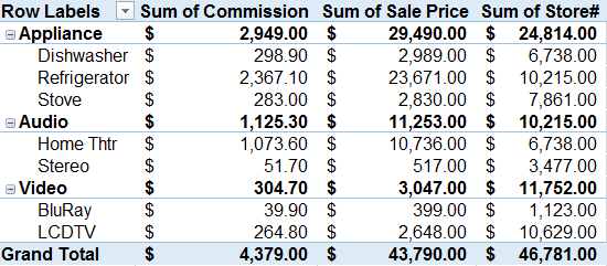
• Which items generate the most sales and commissions:

Edit Your Table

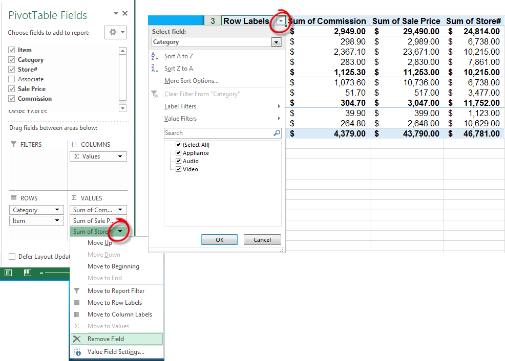
When you choose a recommended PivotTable, you might not get exactly what you were looking for. In the last table, for example, we do not need a “Sum of Store#”. To edit your PivotTable:

1. Click anywhere in the PivotTable to open the PivotTable Tools contextual tab and the PivotTable Fields pane.
2. Add or remove fields in the Fields pane to include exactly the information you need. We would select Remove Field for the “Sum of Store#” in our example.
3. Filter data to include only the items you want. Click the dropdown filter arrow to see a list of the fields in the column or row you are working with. Un-check any fields you do not want to appear in the table.

With the Quick Analysis Tool, you can create a PivotTable with a few simple clicks, then make small edits to get exactly what you need. This method recognizes that it’s easier to edit a table that is almost ready than start from scratch.