Learn How to Find Duplicates in Excel and Either Use or Remove Them

It’s a common scenario: Data is combined from multiple sources, records are entered by multiple users or you simply have multiple transactions with the same information. The end result is that you need to find and manipulate duplicates. Excel gives you several ways to do this, depending on your data and what results you are after. This article covers three of those methods and a scenario in which you might use them. The following steps apply to Excel 2007-2013. Images were taken using Excel 2013 on the Windows 7 OS so the specific steps may vary based on your version.

Use Advanced Filter

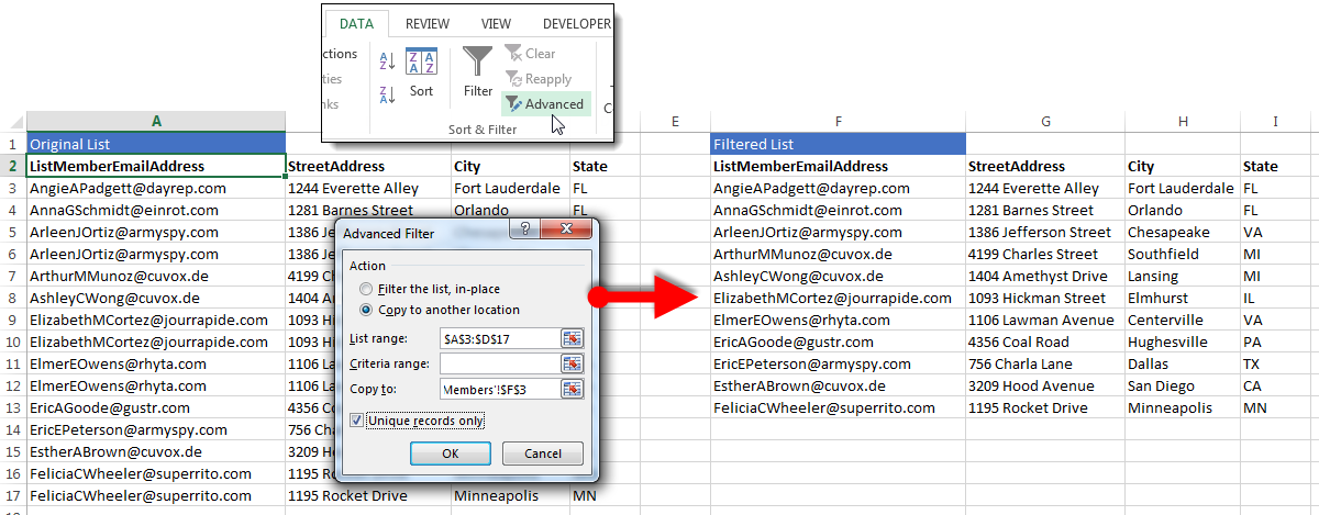
Scenario: We have a list of people who were members of our business association in 2014, and another list of those who were members in 2015. We would like to generate a new list of all people who were members in one or both years and remove the duplicate rows of the members who were in both. With the advanced filter we can do this in one step. To follow using our example, download Find Duplicates.xlsx: Renewing Members

Start by merging the two lists into a new sheet using copy/paste or Excel’s Consolidate feature, etc.

1. Click on any cell with data in your worksheet.
2. Click the Advanced button in the Sort & Filter group on the Data
3. In the Advanced Filter dialog box:
   • Choose the Copy to another location radio button
   • Check to see that Excel has correctly identified the data you wish to filter in the List range: text box and select or correct the range if not
   • Choose a destination for the filtered list in the Copy to This can be on the same sheet or in another sheet.
   • Check Unique records only. This will copy all unique records and only 1 instance of any duplicated record.

Note: This method only removes duplicates when the entire row/record is the same. If you need to identify records that only have some fields in common, use the next method, Excel’s Built-in Remove Duplicates Feature.

Use Excel’s Built-in Remove Duplicates Feature

Scenario: We would like to mail a print postcard to the members of our email mailing list, but have discovered that some have signed up more than once with different email addresses. This means we would send multiple postcards to the same address. We want to remove those duplicate addresses.

Hint! Always start by creating a copy of your worksheet before you begin working so your original data remains safe.

To follow using our example, download Find Duplicates.xlsx: Mailing List

1. Click on any cell with data in your worksheet.
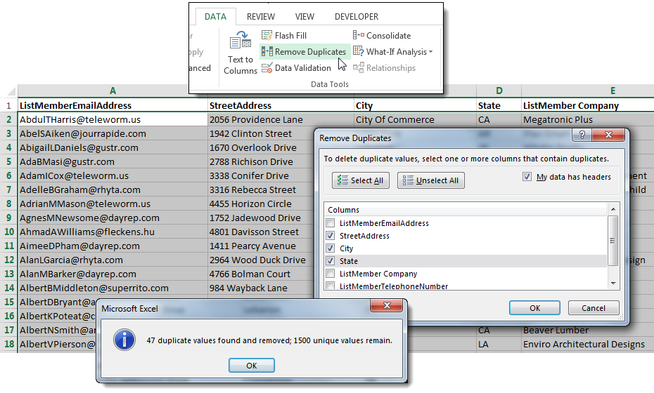
2. On the Data tab, click Remove Duplicates to open the Remove Duplicates dialog box.
3. Put a checkbox by each column that has duplicate information in it. In our example, we want to find identical addresses. (Note: Hit Select All to only remove records that are exactly alike.)
4. Click OK. Excel will automatically find and remove all but the first row of matches that contain the same information.

Use a PivotTable

Scenario: You have a spreadsheet listing all attendees at a convention you are hosting. You want to know how many people from each company are attending so you can offer a discount to those bringing 5 or more employees.

To get a count of rows that have duplicate information, in this case – the same company name – a PivotTable offers you a very quick way to view and then manipulate that information.

To follow using our example, download Find Duplicates.xlsx: PivotTable

1. Insert a new, blank PivotTable into your workbook.
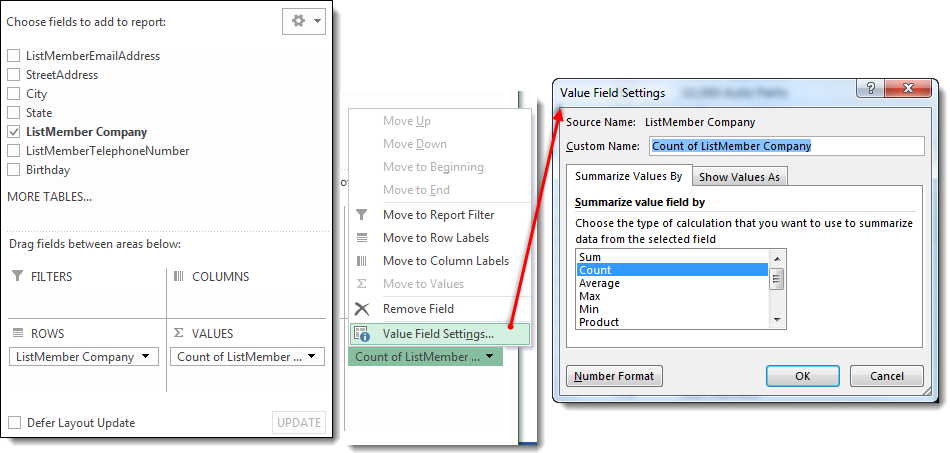
2. In the PivotTable Fields pane, choose the field that contains duplicates and place it both in the Rows area AND in the Values The Summarize setting should default to Count but if it does not, open the Value Field Settings dialog box and choose Count from the selection box. The result will be a PivotTable that shows each company in the left column and the number of times that company appears in the column in the right column. This is the number of attendees from each company.
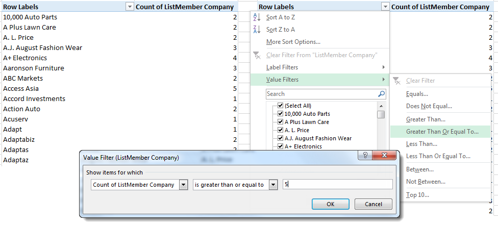
3. Since we want to only see those companies that have 5 or more attendees, we will need to add a filtering step. Click on the filter arrow on the Row Labels
4. Choose Value Filters and then the appropriate criteria, in this case Greater Than Or Equal To.
5. Fill out the details of your criteria in the Value Filter dialog box and click

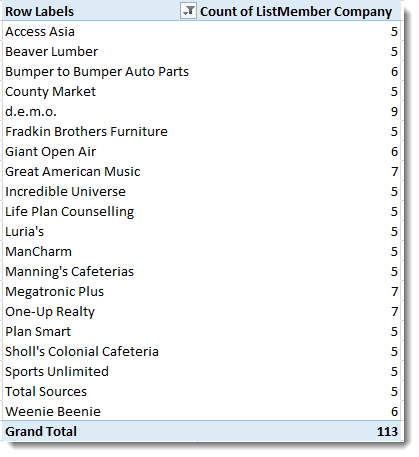
Our PivotTable will now only show those rows that have 5 or more duplicates in the ListMember Company column on the original table.

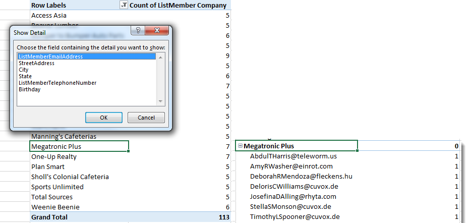
A very useful feature of a PivotTable is that you can then “drill down” into the data behind the summary. Double-click on any of the “5 or more” companies to see attendee detail for that company, for example.

Though you will have different data and different scenarios, one of the three above techniques can help you get started on the solution you need when working with data that has duplicate information.