How to Use Slicers in Excel 2010 and 2013

Excel’s Slicer Filter was added in Excel 2010 and enhanced in Excel 2013. This useful feature is excellent for viewing and comparing varied combinations of your data with a simple click. Something like a cross between a button and a filter, Slicers have become a prized tool for analyzing large data sets in dashboards and reports. This article will demonstrate how to create a slicer in both 2010 and 2013 versions of Excel.

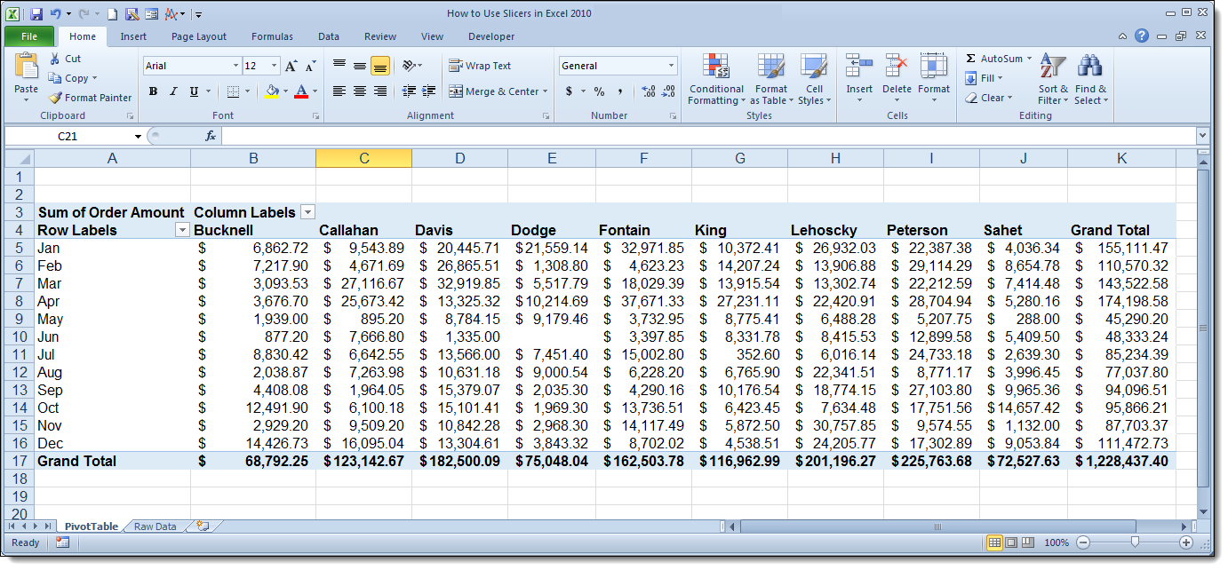
Our example data includes monthly totals for a large sales team. The number of team members makes it difficult to compare performance among them. We will use slicers to narrow our view and filter the table without having to click on tiny filter arrows and select from cumbersome drop-down lists. To follow using our example, download How to Use Slicers in Excel

For this exercise, begin by creating a PivotTable from your raw data with the set of fields you wish to analyze. In Excel 2010, you can only apply slicers to PivotTables, but 2013 will also let you add slicers to data tables.

Adding Slicers to a PivotTable in Excel 2010

The following images were taken using Excel 2010 on Windows 7.

1. Click on any cell within the PivotTable for which you want to create a slicer. This will activate the PivotTable Tools contextual tab.
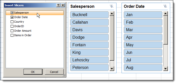
2. In the Sort & Filter group in the Options tab, click on the Insert Slicer combo button. The Insert Slicer dialog box will open.
3. In the Insert Slicers dialog box, click the checkboxes by the PivotTable fields you want to filter by. A slicer will be created on the same worksheet for every field that you selected.
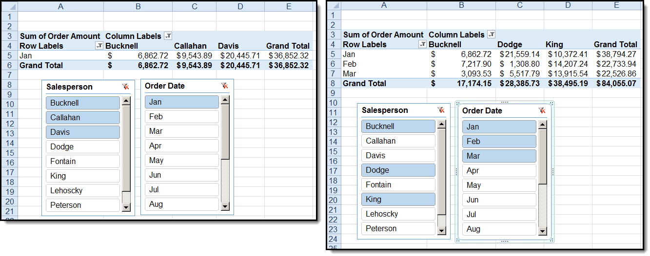
4. In the slicer window, click on any item on which you want to filter. If you want to view more than one item at a time, hold CTRL key and click multiple items.

Adding Slicers to a PivotTable in Excel 2013

The following images were taken using Excel 2013 on Windows 7.

1. Click on any cell within the PivotTable for which you want to create a slicer. This will activate the PivotTable Tools contextual tab.
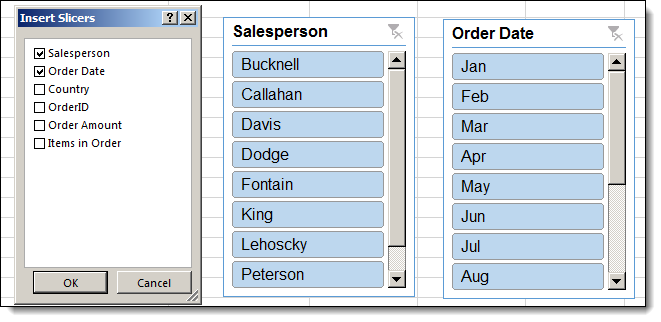
2. In the Filter group in the Analyze tab, click on the Insert Slicer button to open the Insert Slicers dialog box.
3. In the Insert Slicers dialog box, click the checkboxes by the PivotTable fields you want to filter by. A slicer will be created on the same worksheet for every field that you selected.
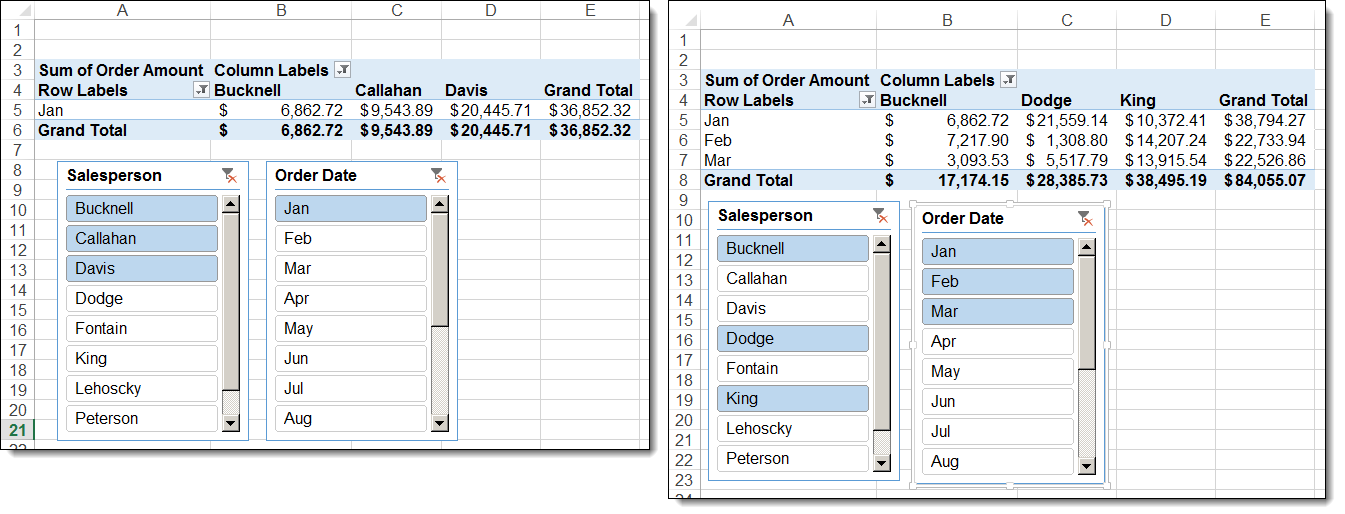
4. In the slicer window, click on any item on which you want to filter. If you want to view more than one item at a time, hold CTRL key and click multiple items.

Add a Slicer to a Table in Excel 2013

In Excel 2013, you can add slicers to regular tables. Use the Raw Data tab in the How to Use Slicers in Excel workbook to try it yourself.

Your data will need to be formatted as a table with row headings. Then, click anywhere in the table to activate the Table Tools contextual tab. Click the Design tab and then the Insert Slicer button to open the Insert Slicers dialog box.

Delete a Slicer

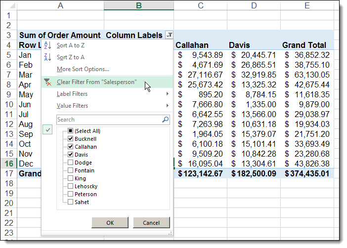
First, clear all filters by unselecting the slicer fields. Then, select the slicer object and hit the delete button. If you do delete a slicer with filters chosen, your table will not refresh. You will have to manually clear any active filters by clicking the filter icon and selecting Clear Filter from the dropdown menu.

Slicers let you create truly interactive tables. They are perfect for live presentations when you need to answer questions about specific “slices” of your data on the fly. And because of the visual nature of the slicer buttons, you’ll always know what you are looking at.