Interactive Excel Charts: Create a Chart Selector

More and more data has led to more and more opportunities to present it in visually understandable ways. However, it can get frustrating having to navigate through a large workbook, just to find the exact chart you need. In this tutorial, you’ll learn how to create an interactive chart selector. If you aren’t familiar with Excel, creating named ranges, formatting charts, or using form controls, you may find these instructions challenging.

Download InteractiveExcelCharts.xlsx and follow along.

Step-by-Step

1. Set up your worksheets and check your data.

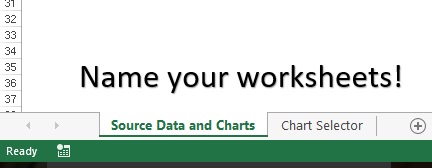
Name the worksheet where you will place your charts, data, and other source information you’ll use for the chart selector. Make sure your charting data is in good shape:

• No completely blank rows or columns
• Each column has a column title
• Columns contain consistent data, such as all currency values, all percentages, all dates

2. Format/Create your charts.

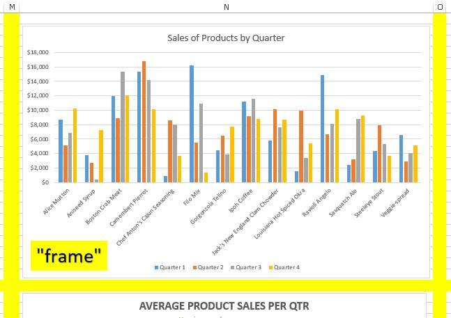
In the sample, we have already created six charts. Creating the interactivity later is easier if all charts are on the same worksheet. Place the charts in their own column and position so that there is at least one row between each chart and on either side, creating a frame.

3. Create a named range for each chart.

Select the cells in which the chart is located (for example, N1:N24 for Chart1), then name the range. We named ours Chart1 through Chart 6.

4. Create chart selection list and name the range.

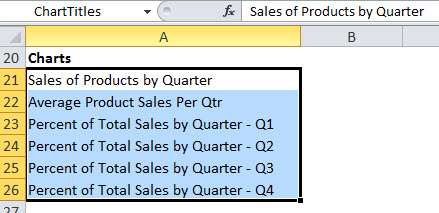
Create a list containing each chart’s title, being sure that the first name corresponds to Chart1, the second to Chart2, and so on. Let’s create a named range with the titles selected and call it ChartTitles.

5. Create combo box control.

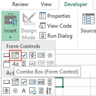
Now to create our interactive chart selector worksheet, we need a way to tell Excel what chart to show. Add a new, blank worksheet and name it Chart Selector. Next, we will insert a form control called a combo box. It is a button that acts as a dropdown list for us to select our chart. This button is found in the Controls group on the Developer tab. Once selected, drag the crosshairs to draw it in the worksheet. Don’t worry too much about the size or dimensions of the box. You can adjust it later.

6. Configure combo box control.

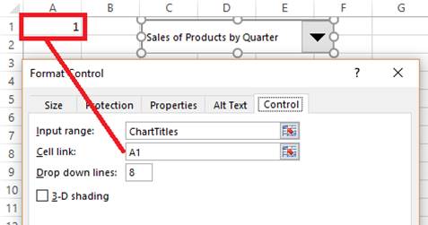
To make the combo box show us our chart titles when we click the arrow, we’ll need to set the properties. Right-click the combo box and choose Format Control in the pop up menu. The Form Control window will open. It’s here that we want to tell it to find that named range we made for our chart titles. Just type the name into the Input Range field. Click in the Cell link field and choose any empty cell in the worksheet. Click OK. Now you’ll notice that the dropdown arrow reveals your list of chart titles. And choosing one, changes the number in that cell link cell (that’s A1 in our example).

7. Correlate chart title list position with the chart named range using the CHOOSE function.

Now that you have created a cell link, we can tell Excel to show a chart based on that chart number. Go to the Formulas tab and click on the Name Manager button. When the Name Manager window appears, choose New… We’ll name it ChartChoice. Using the CHOOSE function, create a formula that reads what’s in the cell link cell and associates it with a chart’s named range.

It should look something like this:

=CHOOSE(‘Chart Selector’!$A$1,Chart1,Chart2,Chart3,Chart4,Chart5,Chart6)

8. Link chart named range to report location.

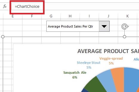
Now, to link this to actually showing a chart, click the dropdown arrow in the name box in the upper left corner and click the first chart range. Copy, then paste it on the Chart Selector worksheet as a linked picture. Look up in the formula bar and you’ll see a formula representing the pasted chart. Change this to an equal sign followed by the new range name you created in step 8 above. In our example it was ChartChoice.

Test out your new creation! Select a chart and watch it pop up.

Finishing Touches

Declutter the appearance: Turn grid lines off on both worksheets to get rid of messy overlapping grid lines. And, hide the column that has your Cell link cell.

Protect your hard work: To make sure that nothing gets rearranged and that the workbook just allows the user to choose a chart, hide all the worksheets except the Chart Selector. Just right click the worksheet tab and choose hide.  Now, unlock the Cell link cell, so that it can still be changed by the combo box form control. Finally, protect the sheet (password is optional). Uncheck the Select locked cells check box. This will allow users to only choose a chart and see their choice.

Download the solution file to see how you did! InteractiveExcelChartsSolution.xlsx