Learn about the Excel Find Formula
Sometimes getting valuable or actionable information out of your data is a bit like going on a treasure hunt: You spend a lot of time solving puzzles and putting together a “map” of formulas that will hopefully lead you to the goldmine of information hidden inside.
The FIND function, and its close cousin SEARCH, is a function that can move you closer to the treasure of useful information, especially when combined with other functions.
Let’s start by understanding the basic FIND syntax. FIND will locate a specified text string within a second text string then return the number of the result’s starting position. These steps will apply to Excel 2007-2013. Images were taken using Excel 2013 on the Windows 7 OS.
SYNTAX: FIND(find_text, within_text, [start_num])
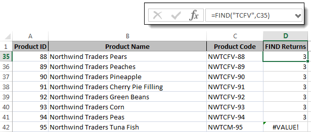
In the example, we have created a formula that will search for the text string TCFV in the Product Code cell. A 3 is returned in row 35-41 because TCFV is found beginning at the 3rd character of the Product Code. An error #VALUE! is returned in row 42 because TCFV is not found in C42.
It is important to note that FIND is case sensitive. If we had searched for “tcfv” instead of “TCFV” as in the next example, no results would be found.
This is when FIND’s close cousin SEARCH comes in handy. SEARCH is not case sensitive and allows wildcard characters in the find_text argument.
This function helps us find strings of text within other strings of text. Now let’s look at more ways to build upon this function to create something truly useful.
Combine FIND with IF and ISERROR to create True/False results
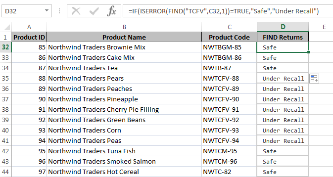
Often when you search for text you want to display a result based on whether, or not, a match was found. In this example, the resulting formula lets us know that all products with the string TCFV in the Product Code are under a recall, and all other products are safe.
If we were to describe this formula in natural language, it might go: If an error is produced because the FIND function did NOT find the string “TCFV”, then display the text “Safe”, otherwise display the text “Under Recall” because the string was found.
There are many potential uses for this technique that lets you choose specific actions based on whether your text string is found.
Combine FIND with MID function to return only the information you need
If you have data that is a long string of characters and only a subset of those characters is useful to you, then you can use the MID function to pull out only those that you need, such as the two numbers that always follow a dash in our Product Codes.
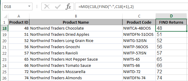
Sometimes, however, your data is not consistent enough to simply tell Excel to “return the 6th through the 8th” character. Our Product Codes in the next example always begin with “NW” but there are sometimes four and sometimes two more characters before the dash. So how could we return only the two characters after the dash with the MID function? SYNTAX: MID( string, start,[length] )
Instead of specifying a start character, we can use the FIND function as the start argument. FIND will return the character location of the dash. We will add +1 to indicate that we want the MID starting place to be one after the dash’s location.
What are some other ways you have used the FIND function?


