Nesting Functions in Excel – A Tutorial for Beginners

Most of us begin using Excel by creating simple worksheets that organize data and perform simple calculations. Then, we might dabble with some of Excel’s many pre-set functions for more complex calculations. You know you’re a real Excel addict, however, when you start thinking How can I crunch my data even more efficiently? This means you’re probably ready to combine your functions and create more complex formulas. Here is a quick tutorial for nesting functions without getting lost:

What is nesting?

Nesting refers to using a function as one of the arguments inside another function.

When do you use nesting?

Nesting functions is useful when you need to make several calculations to get to your desired answer, but don’t need to see the results of those steps as you go.

How do I keep my nested functions straight?

If you’ve ever looked at someone else’s worksheet and felt your eyes glaze over at the long strings of numbers, cell references and function names, you’re not alone. It takes practice to “read” complex formulas. Here are a couple of quick tips:

• Know your function’s arguments – Knowing that the IF function has 3 arguments separated by commas (criteria, if true return, otherwise return) will help you sort out what each nested function is meant to accomplish.
• Count your parenthesis – Just like in math equations and computer programs, parenthesis keep instructions organized and tell you what order the calculations are performed. When creating nested functions, you will need to make sure that all of your open parenthesis have closing parenthesis and that they’re in the right place!
• Don’t work left to right, work inside out! – It’s tempting to try to build a complex nested formula by starting at the beginning of the line. Instead write the internal functions first, then place them as a unit into the arguments of the outer functions.

Let’s do an example. To follow along, download 05-Nested Function Tutorial.xlsx

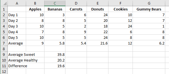
Our worksheet shows six food items – 3 healthy and 3 sweet – and how many students chose each for their afternoon snack over 5 days.

We want to know how many more students, on average, chose sweet snacks instead of healthy snacks.

To make that calculation we will need the following information. To answer the question without nested functions, you could use multiple additional cells and the formulas in the example below:

• Average of each snack: =AVERAGE(B2:B6), =AVERAGE(C2:C6), =AVERAGE(D2:D6), and so on
• Average of each kind of snack: =SUM(E7:G7) & =SUM(B7:D7)
• Difference between healthy average and sweet average: =C9-C10

See Multiple Cells Tab

As you can see, each calculation is contained in its own cell, and the final “Difference” formula is built on the results of those cells. If, however, we don’t care about the average per snack or snack type, and ONLY want to see the “Difference”, we can nest our functions into one long formula.

Let’s do it first in plain language. To calculate the difference, we’ll need to subtract the total average of healthy snacks from the total average of sweet snacks:

• Difference = (average number of sweet snacks) minus (average number of healthy snacks)

The average number of sweet snacks is calculated by adding together the average number of each individual snack in the category. Our formula will be:

• Average number of healthy snacks = (Average of Apples + Average of Bananas + Average of Carrots)
• Average number of sweet snacks = (Average of Donuts + Average of Cookies + Average of Gummy Bears)

Working inside-out, now fill each snack category parenthesis with the correct function:

• • Average number of healthy snacks = SUM(AVERAGE(B2:B6), AVERAGE(C2:C6), AVERAGE(D2:D6))
  • Average number of sweet snacks = SUM(AVERAGE(E2:E6), AVERAGE(F2:F6), AVERAGE(G2:G6))

Notice that the parenthesis around the SUM arguments stack up at the end. You need both end parenthesis to “close” the AVERAGE function and the SUM function.

Now, using these complete functions, we can now put them in the difference equation, for a final result of:

=SUM(AVERAGE(E2:E6), AVERAGE(F2:F6), AVERAGE(G2:G6))– SUM(AVERAGE(B2:B6), AVERAGE(C2:C6), AVERAGE(D2:D6))

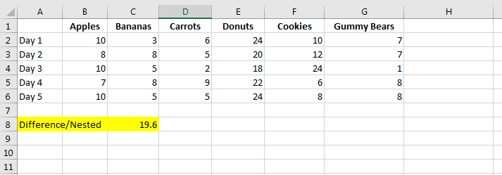
When you plug in the above, you get the same result as the first formula, but you don’t need to have any of the additional helper cells!

See Nested Functions Tab

This example is probably a bit much for a simple problem, but it should illustrate the benefits and techniques of nesting functions to create more complex formulas without adding additional clutter to your sheets.

What are your tricks for working with nested functions without getting “lost in the parenthesis”?