Tips for Creating Perfect Pivot Tables with a Macro

Once you’ve harnessed the power of PivotTables, you probably find yourself looking for ways to use them all the time. The same is true of macros – convenient shortcuts that make your life easier! But have you tried to combine the two?

Unless you are turning the exact same format and type of data into PivotTables over and over, it might not make sense to record a macro that only works against one spreadsheet. However, there are some ways a macro can be really helpful when adjusting your PivotTables to get them to look consistent and useful.

Here are two tips to make creating and editing PivotTables easier. Images in this article were taken using Excel 2013 on the Windows 7 OS. Specific steps to complete the tips will vary based on the version of Excel 2007-2013 being used.

Turn your data into a table

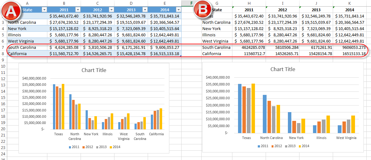
If not already, turn your data into a table instead of raw data (and give the table a name in the Properties group on the Design tab). As of Excel 2007, tables offer you the great benefit of organizing information in a way that is easily updatable. For example, if you have created a Chart based on a table and then add rows of information to the table, the chart will automatically refresh, as it has done in example A.

In example B, the same two highlighted rows of information were added to the data, but the chart did not refresh. You would have to click the Select Data button and manually add the new rows to the data range.

To follow using our example, download Excel Macro PivotTable

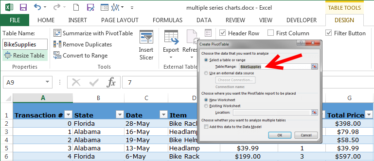
The same convenience applies to PivotTables. If your information is in a Table, select the Table name when you are creating it and then you won’t have to constantly change the Table’s range when you add rows to the data.

Determine your “common” settings

Do you always turn off Subtotals? Do you have a custom, corporate PivotTable Style that you always select each time you create a new PivotTable?

To take advantage of macros and still leave yourself enough flexibility to use the macro on different sets and layouts of data, think through all those extra clicks you perform for almost every PivotTable you create. Then, to create your time-saving PivotTable Macro follow these steps:

1. Put your mouse cursor inside the data table before you record the macro.

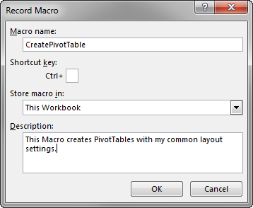
Start recording macro.

2. Click Insert > PivotTable
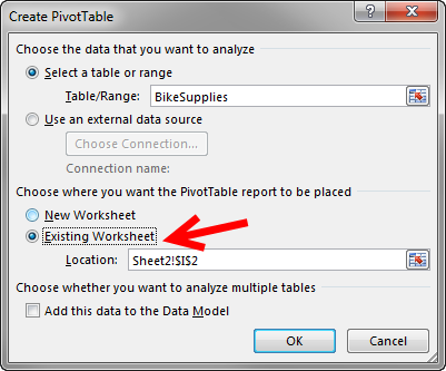
3. Make any of your usual changes to the Create PivotTable dialog box, such as changing where it will be placed.

Note that because your data is in a table, and that you clicked inside the table before you created the PivotTable, the Table/Range defaults to the data you want, even if the area is different each time you run the macro.

4. Click OK. Excel will then open the PivotTable Fields pane and put a placeholder Report in the place you defined in the Create PivotTable dialog box.
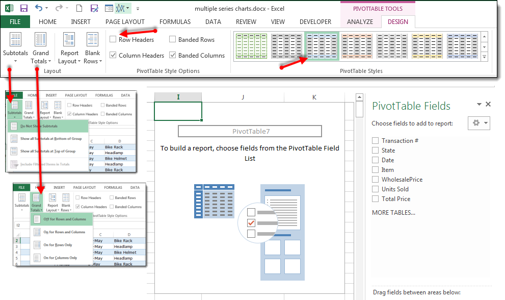
5. BEFORE you choose fields and create your report, make the other layout changes you would like captured in your macro, first. These changes might include:
   1. Changing Subtotal and Grand Total defaults
   2. Turning Row and Column headers off or on
   3. Choosing a PivotTable style

6. Once all of your layout changes have been captured, STOP the macro.

Now you can create your report to meet the specific needs of the data, but those common annoying clicks will be handled in a flash the next time you are ready to create a new PivotTable. Just click anywhere inside the table that contains your data, and then run your macro.

AND, because your source data is in a table, just add new rows as needed to your data, hit Refresh on your PivotTable and the new information will automatically appear.